Paraxial Beam, Gaussian Basics
ECE
5368/6358 han q le - copyrighted
Use solely for students registered for UH ECE
6358/5368 during courses - DO NOT distributed (copyrighted
materials)
Utility
0. Introduction
Why study Gaussian beam?
- Historically, long before the ubiquitous diode lasers, early
lasers were often gas lasers
- Gas lasers are built with macroscopic external cavity with
concave mirrors
- Gaussian beam is the output profile these gas lasers
(http://en.wikipedia.org/wiki/Gaussian_beam)
- Understanding Gaussian beam is essential to
design these laser cavities (Hermite-Gaussian profiles are the
transverse mode of most of these lasers), as well to use of these
laser beams outside the cavity.
- More than just for the practical reason dealing with lasers, the
mathematics of Gaussian beam is manageable and instructive to gain
insight and understanding of the basics of coherent light
propagation, hence it is a worthwhile topic in itself.
- Concepts such as beam waist and beam divergence are basic to any
beam and light propagation in general. As a light beam undergoes
transformation through optics, especially Fourier optics (since
the Fourier transform of a Gaussian is also a Gaussian), it is
important to determine its properties, and Gaussian beam provides
a very useful approximation even for non-Gaussian beams.
- Nowadays, most common coherent light beams are the outputs of
diode or semiconductor-waveguide laser or optical fiber. They have
transverse mode profiles that are not necessarily Gaussian, but
simple Gaussian-based formula can still be used as a rough
approximation or quick rule-of-thumb estimation. The calculation
with Gaussian beam is simple and easy to do.
1. Paraxial approximation for Gaussian beam (can skip)
In the below, you can skip all sections with heading in light gray background.
Earlier, we review 2D Gaussian beam. Here, we will study 3D (most common) Gaussian beam.
A beam coming
out from a small spot acts like a spherical wave. A beam coming
out from a large spot acts like a plane wave. How do we account
for these extreme behaviors with a single, simple formulation? We
don't want to have to use a different "approximate" for each
situation.
Beam propagating along an axis: paraxial beam. The solution can be
separated in two parts: traveling logngitudinal part (along the
axis) and lateral part. In free space, an important type of
paraxial beam is Gaussian beam.
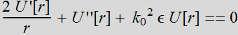
Hemholtz's
equation:
![]() ==>
==> ![]()
Separate by part would suggest ![]() .
But we have to remember that at infinity, the plane wave approx.
is good over a small region (compared with the beam spread), but a
spherical wavefront is the correct approximate over the entire
beam.
.
But we have to remember that at infinity, the plane wave approx.
is good over a small region (compared with the beam spread), but a
spherical wavefront is the correct approximate over the entire
beam.
1.1 Spherical wave review
![]()
![]()

For spherical wave without angular dependence:
![]()
The Helmholtz Eq.:
There are two
solutions:
 or
or 
for radiating wave or collapsing wave: these wave have singularity
at origin.
1.2 In cylindrical coordinate

![]()
1.2.1 Exact solution: Bessel J0
The equation
becomes:
![]()
Change variable: for ![]() > 0:
> 0:
![]()
![]()
![]()
![]()
1.2.2 Review Bessel function
![]()
The solution is
Bessel ![]() that is not singular at 0,
that is not singular at 0, ![]() diverges at zero.
diverges at zero.
Bessel beams are the only type of beam that does not change shape
as it travels! But a pure Bessel beam extends to
infinity and goes down very slowly ![]() .
These are not common beams.
.
These are not common beams.
![]()
![]()
1.2.3 Linear superposition solution
General solution
is then:
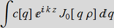 where
where ![]()
What if ![]() = 0?
= 0?
![]()
![]()
The non-plane
wave solution ![]() is neither regular at zero or infinity: this is not a physical
meaningful solution for a finite beam at ρ=0.
is neither regular at zero or infinity: this is not a physical
meaningful solution for a finite beam at ρ=0.
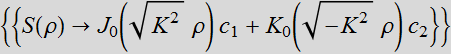
What if ![]() <0?
We define
<0?
We define ![]()
The equation:
![]()
has solution Bessel I or Bessel K: neither one is regular: I is
infinite at infinity, K is infinite at zero.
![]()
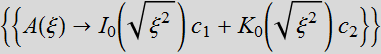
![]()
![]()
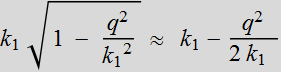
This is a
problem: what if the wavefront at the plane z=0 has q component up
to ∞? We notice that if q > ![]() ,
the only way the Helmholtz equation is satisfied is that the
z-dependence plane wave is:
,
the only way the Helmholtz equation is satisfied is that the
z-dependence plane wave is: ![]() where
where
![]() .
This is an acceptable solution in either + z or - z direction as
long as it goes to zero at infinity: We call this evanescence
wave. It is meaningful only for a short distance of z. Thus, for a
propagating wave solution, this component vanishes eventually and
can be ignored. But it can be important at near field solution,
which is the basis for near field spectroscopy.
.
This is an acceptable solution in either + z or - z direction as
long as it goes to zero at infinity: We call this evanescence
wave. It is meaningful only for a short distance of z. Thus, for a
propagating wave solution, this component vanishes eventually and
can be ignored. But it can be important at near field solution,
which is the basis for near field spectroscopy.
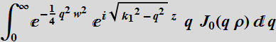
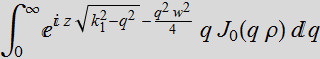
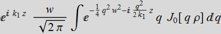
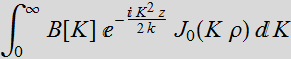
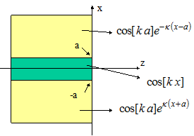
1.3 Gaussian beam paraxial propagating solution
1.3.1 Gaussian
The general
propagating wave solution is a linear superposition of Bessel
beams.
How do we form a linear superposition of Bessel beams?
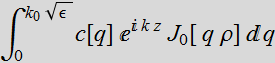 where
where
![]() (1.3.1)
(1.3.1)
Notice that we have a cut-off at ![]() .
Near this value,
.
Near this value, ![]() is nearly constant: the wave is not propagating in the z
direction. The paraxial solution for typical laser beam should
have
is nearly constant: the wave is not propagating in the z
direction. The paraxial solution for typical laser beam should
have ![]() and q very small.
and q very small.
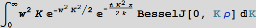
We have formed a
linear superposition of plane wave. We'll do the same for Bessel
waves; but we need to assume certain function c[q]
. Obviously, c[q]
can not be finite at q=0: we have singular solution! so we'll
choose ![]() .
.
![]()
What we find,
interestingly is that by choosing ![]() ,
along with paraxial approximation, we get a Gaussian profile.
,
along with paraxial approximation, we get a Gaussian profile.
![]()
Thus: 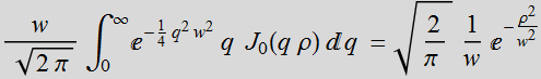
We see that with the approximation 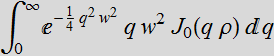 with the integration limit to infinity instead of
 ![]() ,
we have a closed-form Gaussian solution. This is the Gaussian
profile at z=0 that we want! To extend this approximation to any
z, we write:
,
we have a closed-form Gaussian solution. This is the Gaussian
profile at z=0 that we want! To extend this approximation to any
z, we write:
![]() =
=  : this is the paraxial approximation.
= 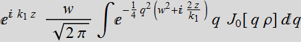
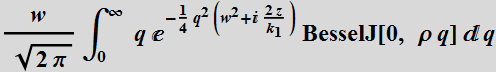

The approximated
solution is:
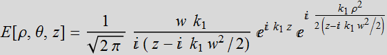
=
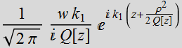 (1.3.2a)
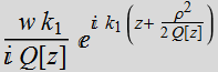
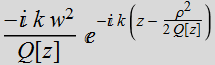
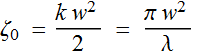
where  (1.3.2b)
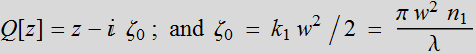
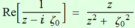
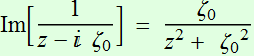
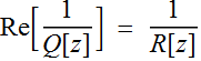
What is the meaning of this Q[z]
term?  :
defined as Rayleigh range. So Q[z]
is a quantity of unit length, but has an imaginary component:
:
defined as Rayleigh range. So Q[z]
is a quantity of unit length, but has an imaginary component: ![]()
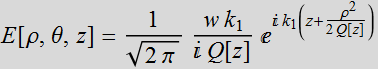
To include the time:
 (1.3.3)
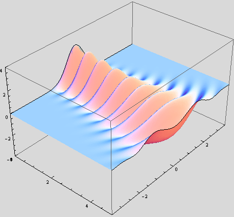
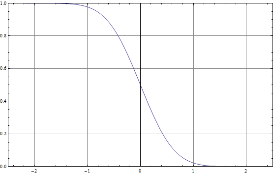
Let's plot electric field (or H field):
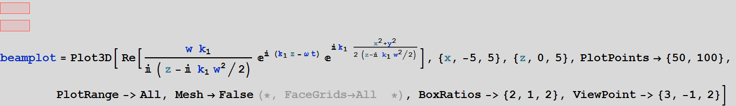
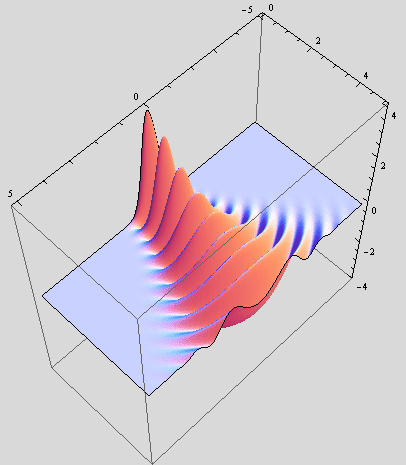
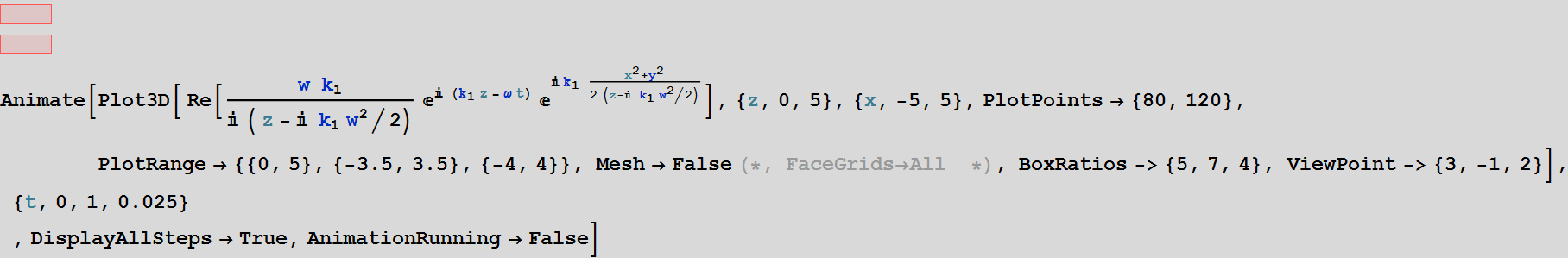
Below is a code to use if the computation is slow:
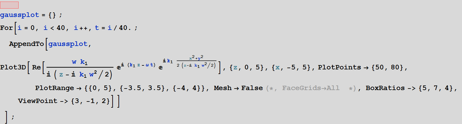
![]()
Gaussian beam solution (in spite of being a paraxial approximation) is very good in describing circularly symmetric laser beam behavior: from tightly focussed, highly divergent beam to plane-wave-like beam.
Even if the beam is not circularly symmetric, but elliptic with x, y axis, it can still be used with separate x and y profile and all the key properties apply.
1.3.2 Phasefront
From the
Gaussian beam description:
 (1.3.2a)
where 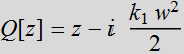 (1.3.2b)
We write
separate the phase and the amplitude:
 =
=
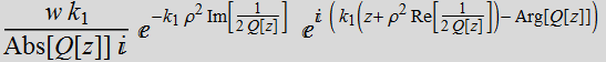
Amplitude: ![]() (1.3.3)
(1.3.3)
Phase: ![]() (1.3.4)
(1.3.4)
The constant
phase front (cophasar surface) is:
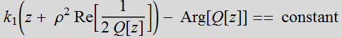 (1.3.5)
At z = 0,  =0, Arg[Q[z]]=
constant, so the phase front is a plane: it is independent of ρ.
=0, Arg[Q[z]]=
constant, so the phase front is a plane: it is independent of ρ.
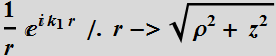
What about at
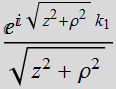
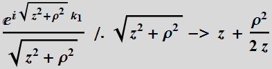
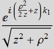
farfield, where z-> ∞?
Using: 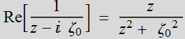 ;
; 
As z-> ∞, 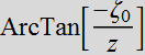 ->
-0, the phase front is given by
->
-0, the phase front is given by
~
z + ![]() =
=
![]() =r
= constant: this is nearly a spherical wavefront.
=r
= constant: this is nearly a spherical wavefront.
Gaussian beam can describe both planewave-like behavior at near field and give spherical-wave-like at farfield. It is a highly versatile model for coherent optical beams (laser beam) that can be used in many calculation.
1.3.2 Compared with spherical wave
Gaussian
beam:  where:
Spherical wave: 
![]()
Note that:
Spherical wave in paraxial approx 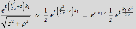
Gaussian
wave 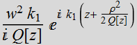
If we change z-> ![]() for the paraxial spherical wave, we obtain:
for the paraxial spherical wave, we obtain:
which is the Gaussian beam solution. The term 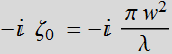 acts
as if it is a virtual point of origin, instead of z=0, it is at
acts
as if it is a virtual point of origin, instead of z=0, it is at ![]() .
.
From this perspective, Gaussian beam acts like a spherical wavefront originating from a virtual point. It should be remembered that Gaussian beam is only an approximated solution. We obtain it by solving the exact Helmholtz equation. Then, we can also ask: is there an approximated Helmholtz equation that gives Gaussian beam as an exact solution?
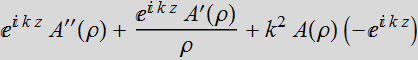
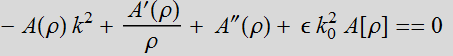
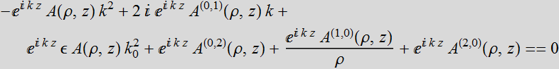
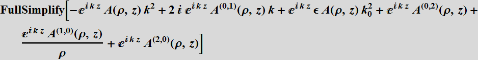
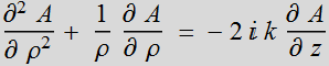
1.3.3 Paraxial Helmholtz equation
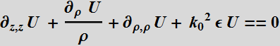


![]()
Remember that we
have the equation:

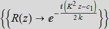
Now, we will let ![]() :
:
![]()
 .
.
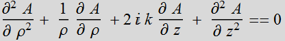
A[ρ,z] is the envelop function superimposed on the plane wave ![]() .
We assume that the wave is very close to plane wave, then the
function A[ρ,z] is slowly varying with respect to z. If so, we can
drop
.
We assume that the wave is very close to plane wave, then the
function A[ρ,z] is slowly varying with respect to z. If so, we can
drop  and obtain:
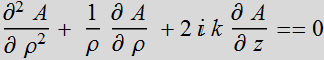 .
Here we have reduced the equation to the first order of z.
.
Here we have reduced the equation to the first order of z.
 .
Now we can solve by part:
.
Now we can solve by part:
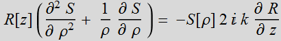 or:
or:
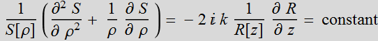
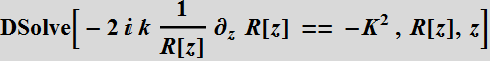
![]()
If K is real
positive, the general solution is:
Choose: B[K]= ![]()
We have the
exact solution:  =
=
Summary
Gaussian beam acts like a the paraxial approximation of a
spherical wavefront:  ,
but originating from a virtual point instead of a real point:
,
but originating from a virtual point instead of a real point: ![]() ,
to give:
,
to give: 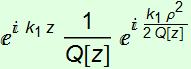 .
.
Gaussian beam is an exact solution to the paraxial approximation of the Helmholtz Eq. and it is an approximated solution to the exact Helmholtz Eq.
2. Important properties of Gaussian beam
2.1 Beam description
From the above
(we drop the subscript 1 from ![]() for simplicity):
for simplicity):
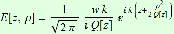 (2.1.1a)
where: ![]() ;
;  (2.1.1b)
Note: we have E[z,ρ] in the unit of  so that the normalized profile:
 is unitless.
Real E has real physical unit, of course. The formula is only for
mathematical convenience. We can also drop the normalization
factor  for convenience. It doesn’t have any special meaning.
We can also
write:
 (2.1.2a)
where: ![]() ;
;

 ;
;  (2.1.2b)
and: 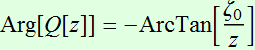 ; (2.1.2c)
What are the meaning of all these formulas? What can we infer?
Source code Demo basic Gaussian density plot
Demo basic Gaussian density plot (run only in Mathematica)
Source code Demo basic Gaussian 3D plot
Demo Demo basic Gaussian 3D plot (run only in Mathematica)
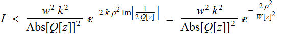
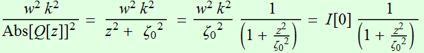
2.2 Beam intensity
2.2.1 Transverse profile
For beam intensity:
 (2.2.1)
 (2.2.2)
It is a Gaussian
profile: 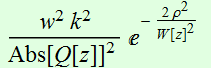
with a beam intensity radius:
 ==>
==>  (2.2.3)
Substitute:
 (2.2.4)
And
with 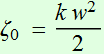
We
obtain: 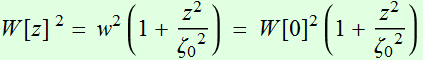 (2.2.5)
The transverse profile of a Gaussian beam
is a Gaussian profile everywhere, with the radius changing as 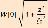 .
We also refer to beam “spot size” as 2 times the beam radius (beam
diameter).
.
We also refer to beam “spot size” as 2 times the beam radius (beam
diameter).
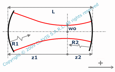
Gaussian beam does not originate from a point: there is no such thing as a point source of light, but there is a place where the Gaussian beam has the smallest profile. The smallest beam radius is called beam waist: W[0]. (see note above also that shows that the point source of a Gaussian beam is a complex number)
HW: plot beam intensity
2.2.2 Beam divergence (focusing)
Obviously, at
large z, the beam radius diverges as:
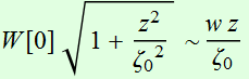 (2.2.6)
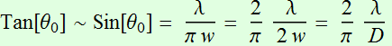
Thus, one can define the divergence angle ![]() with:
with:
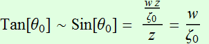 (2.2.7a)
When we deal with small angle: ![]()
Also, with 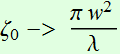
 (2.2.7b).
where D is the “diameter” of the beam. As it turns out, this
formula with a slight modification is almost generic for any beam:
Tan[Divergence angle] =
 (2.2.7c)
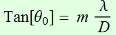
where m is some number
that is a characteristic of a specific beam profile, and which is
![]() for the case of Gaussian. It is 1.22 for example for a top hat
beam. (there is no hard definition for the divergence angle
either, so the number m
is not something fundamental).
for the case of Gaussian. It is 1.22 for example for a top hat
beam. (there is no hard definition for the divergence angle
either, so the number m
is not something fundamental).
Source code
Demo beam divergence 1
For small
angle: 
Often, we talk about beam full
width: 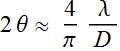 (2.2.8)
An example for non-Gaussian beam: for top hat beam,
instead of  ,
it is 2.44.
,
it is 2.44.
Let’s think: small waist -> large divergence
large
waist -> small divergence
As seen above: waist x divergence =
constant.
This gives rise to the concept of etendue and related to the
definition of brightness.
A similar formula can be used for focusing (see more in section 4).
2.2.3 Longitudinal profile
Again, for the beam intensity above:
 (2.2.1)
 (2.2.2)
But now, we are interested in variation along z.
At
ρ=0 the center of the beam
 (2.2.9)
As z-> ∞, the intensity drops as ![]() as expected for any spherical wave
as expected for any spherical wave
As the transverse profile of a Gaussian
beam gets larger (or smaller), the intensity drops (or increases)
as  (think Lorentzian) by virtue of power conservation.
Source code

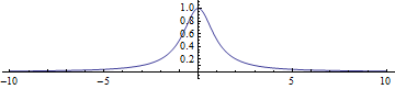
Demo beam intensity along the propagation axis
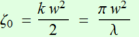
2.2.4 Power conservation
We now can
express the beam intensity
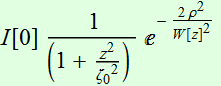 (2.2.10)
where I[0] is the center of the beam intensity at its waist. (the
highest intensity or peak intensity of the beam),
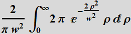
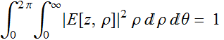
Power is obtained by integrating over all area:
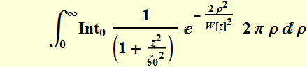
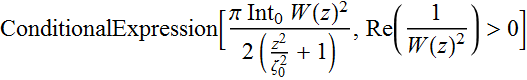
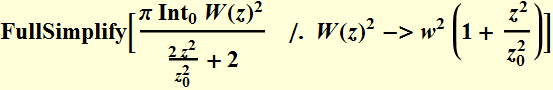
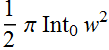
Power
is: 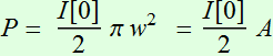 (2.2.11a)
where: ![]() (2.2.11b)
(2.2.11b)
is the beam "area".
We may ask why the factor ![]() ?
It is because I[0] is the peak intensity at the center of the beam
waist:
?
It is because I[0] is the peak intensity at the center of the beam
waist:
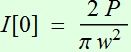 (2.2.12)
The power is an integration over all intensity of the whole beam,
not just the peak. Hence, we can think of (2.2.11a)
as: ![]() (2.2.13)
(2.2.13)
with average intensity 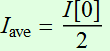 .
Think like the area of a triangle. The area is 1/2 of the height
times the base.
.
Think like the area of a triangle. The area is 1/2 of the height
times the base.
Sometime we
write the beam intensity as:
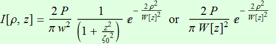 (2.2.14)
2.3 Beam phase
2.3.1 Phase front
Let's look at the beam again:
 (2.1.2a)
where: ![]() ;
;
 ;
;  (2.1.2b)
and: 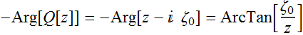 ; (2.1.2c)
The phase term is:
 (2.3.1)
The phase front is defined as:
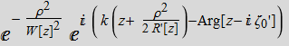
 =constant. (2.3.2)
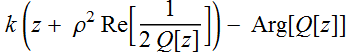
This surface is a function of z and ρ.
What are the meanings of each term? k z
is the plane wave term. 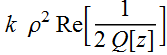 clearly describes the curvature of the wavefront.
 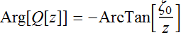 is indepent of ρ, is just a shift that is dependent on z.
If we have a plane wave traveling along a Gaussian
wave of the same ![]() ,
do they traveling in step on the axis?
,
do they traveling in step on the axis?
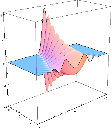
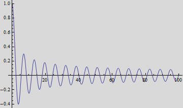
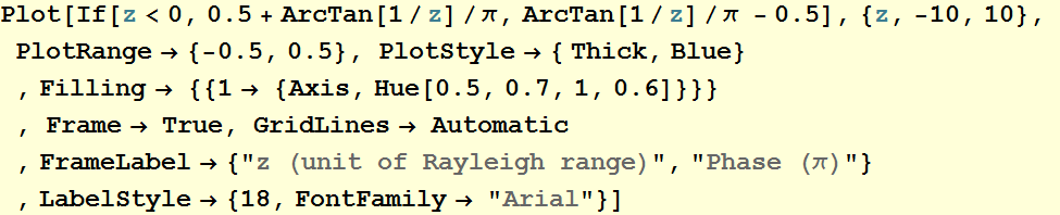
2.3.2 Guoy effect
Not quite. Because for plane wave, it is ![]() ; for Gaussian, it is
; for Gaussian, it is 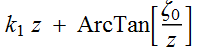 .
So as z goes from -∞ to ∞, The Gaussian differs by a total π phase
shift as shown in plot below. This is called Guoy's effect.
.
So as z goes from -∞ to ∞, The Gaussian differs by a total π phase
shift as shown in plot below. This is called Guoy's effect.
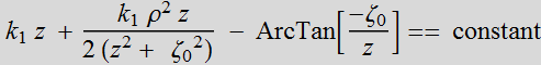
2.3.3 Phase front curvature
Phase front term:
 (2.3.1)
At large z, where z>>ρ, the variation of the term is ~
 (2.3.3)
But this is the equation for a paraboloidal surface:
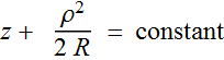 (2.3.4)
where R is the radius of
curvature.
Therefore, we can
define: 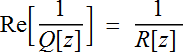 (2.3.5a)
where R[z] is
the radius of curvature of the phase front.
From
(2.1.2b) 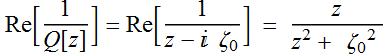 (2.1.2b)
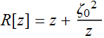 (2.3.5b)
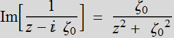
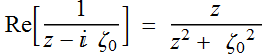
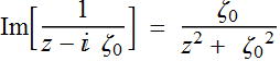
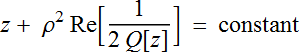
Now we find out what the meaning of  :
:
 ; (2.3.5a)
and 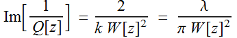 ; (2.3.6)
Thus, we can
write: 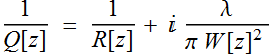 : (2.3.7)
Remember the comparizon of paraxial spherical wave
vs Gaussian: ![]() in spherical becomes
in spherical becomes  in Gaussian. Since
 ![]() in spherical is the radius of curvature, it makes sense that the
Re part of
in spherical is the radius of curvature, it makes sense that the
Re part of  is also the radius of curvature. Remember:
  is NOT the Rayleigh range of the beam. We reserve that term only
for
is NOT the Rayleigh range of the beam. We reserve that term only
for  ,
where W[0] is the beam waist.
,
where W[0] is the beam waist.
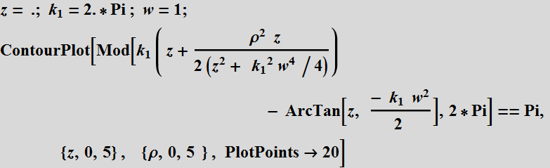
Source code demo phase front
Demo phase front contour (very slow)
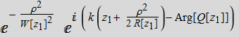
![]()
The  term, where
 ![]() ,
tells us the beam radius of curvature in the real part, and the
beam transverse profile radius in the imaginary part.
,
tells us the beam radius of curvature in the real part, and the
beam transverse profile radius in the imaginary part.
3. Practical techniques to measure Gaussian (or non-Gaussian) beam
Discuss in class only, and for those who really deal with laser beam in the lab.
3.1 Intensity profiling: beam scan method
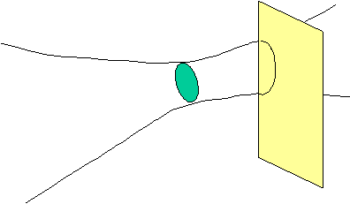
How do we measure the profile of a beam?
Why don't we use things like scanning slit?
Scanning of a Gaussian beam
![]()
![]()
![]()
![]()
3.2 Beam divergence (not at thin lens focal plane)
How do we determine the divergence of a beam? Not
all laser beams are Gaussian (remember that). But first, what is
“divergence”? What is “far field” (FF). Let’s discuss concepts.
The distribution of a beam intensity as a function of angle at
infinity is defined as “far field” (FF). We define a function:
f[θ,φ]. Sometime, it is written: f[Ω], where Ω={θ,φ}.
If we look at a Gaussian beam, the results we saw above is that
the beam profile is
 .
We need to convert this into angle {θ,φ} as z→∞.
.
We need to convert this into angle {θ,φ} as z→∞.
 (also use
 ![]() )
)
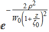
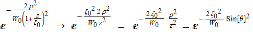
We define 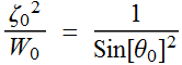 .
Thus:
.
Thus:  :
this is the far field profile function
:
this is the far field profile function
Remember that 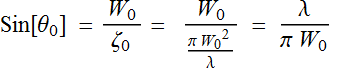 .
.
So now we have a practical question: how do we determine a beam
far-field?
Go out very far, measure the spatial profile, and divide by
distance z? how far? 1 cm? 1 m? 1 km? The key condition
is ![]() :
Rayleigh range.
:
Rayleigh range.
Rayleigh range is the range where the beam diverges very little
and the wavefront is nearly planar: it is where the plane wave
approximation is good.
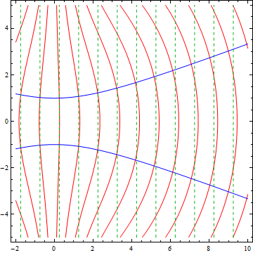
Suppose we have a Gaussian beam with 1-cm diameter (that is, beam waist=0.5 cm), what is the beam divergence? What is its Rayleigh range?
We need to know the wavelength also. Let's λ=0.6328 μm; the beam Rayleigh range is:
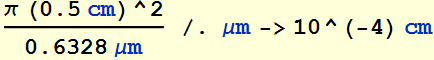
![]()
Suppose we want to measure at a location ~ 10 times
the Rayleigh range, it'll be:
1241 m or 1.2 km! How big is the beam there?
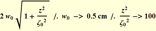
![]()
Clearly, it is not practical to do it this way.
To measure the far field of any beam, we can just
focus the beam with a lens (the reason will be clearer in Chapter
9). We can also then measure the profile after focusing at a
reasonable distance (do not confuse this with measuring the focal
plane of a thin lens that we will learn in Chapter 9).
But then, the divergence we get is just the divergence of the
focused beam, not the original beam! How do we convert? We can
convert for a Gaussian beam using formula in Section 4 below. But
first, let's look at a concept: etendue.
For a beam or an optical system, the product of accepting area and
accepting solid angle is called beam etendue. We can have 1-D
etendue or 2-D etendue. Earlier, we ask a question about Gaussian.
Let's see:
Beam divergence: 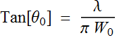 or
or 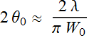 ;
;
Beam waist: ![]() ;
Thus, 1-D etendue =
;
Thus, 1-D etendue = 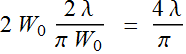 :
constant!
:
constant!
(What is its 2-D etendue?)
So now, if a lens transforms a Gaussian beam into another Gaussian
beam (just of different beam waist), then if we measure the
etendue of one, we knows the etendue of the other! Apply this to
the laboratory exercise.
3.3 Laboratory exercise: ![]() and number of times of “diffraction-limited”
and number of times of “diffraction-limited”
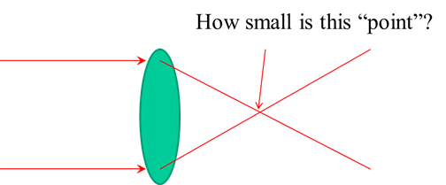
Ever wonder when you focus a beam like laser beam, what is at the focus spot? NOT all beams will give the same spot size even with the same focusing convergence angle! This is the concept of “diffraction-limited”. We will study more in Chapter 8, Diffraction.
Perform a Gaussian beam measurement in the lab and
report your measurement: locate and measure beam waist, measure
divergence angle. Focus the beam with a lens and determine the
beam ![]() .
.
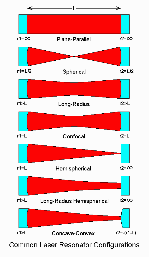
4. Gaussian beam transformation through lenses (and paraboloidal/spherical mirrors)
In practice, rarely any beam is used without any transformation through optics.
Except for integrated optics, which use waveguide to conduct a beam, and the beam profile is determined by the waveguide modes, many systems still use free-space optics.
Even at a very macroscopic level...
The beam profile properties are essential.
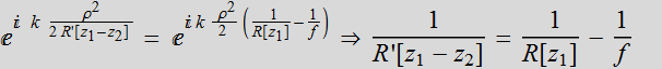
4.1 Review of thin lens and spherical or paraboloidal mirror
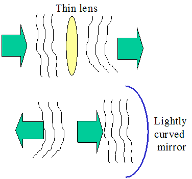
Thin lens and
low-curvature spherical or paraboloidal mirror has an interesting
property: they convert input beam into an output beam with an
approximately paraboloidal wavefront: ![]() for thin lens where f is the lens focal point and
for thin lens where f is the lens focal point and ![]() where
where ![]() is the mirror radius of curvature. (derivation comes from paraxial
approximation). Convention: f>0 for a positive lens, and
is the mirror radius of curvature. (derivation comes from paraxial
approximation). Convention: f>0 for a positive lens, and ![]() < 0 for concave,
< 0 for concave, ![]() > 0 for convex.
> 0 for convex.
Derivation for this comes from ray approximation in which the
phase at location ρ is proportional to ![]() .
(Linked to Simple Optical Elements).
.
(Linked to Simple Optical Elements).
Thus, if a lens is located at location ![]() ,
and the input wave is
,
and the input wave is ![]() ,
then the output wave at the same location is:
,
then the output wave at the same location is: ![]() .
Whatever happens to the wave afterward? at arbitrary z? this is
precisely the interesting property of these optics. In particular,
we will see that Gaussian beam behaves quite nicely with this type
of optics and that is the reason we study it here.
.
Whatever happens to the wave afterward? at arbitrary z? this is
precisely the interesting property of these optics. In particular,
we will see that Gaussian beam behaves quite nicely with this type
of optics and that is the reason we study it here.
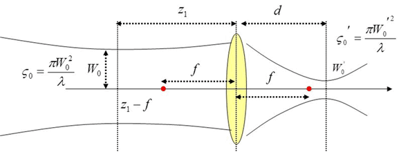
4.2 Gaussian beam after a thin lens. (derivation)
A Gaussian beam remains a Gaussian through a thin lens (or equivalent parabolic mirror) but with a different beam waist location, value, or direction of propagation (the case of mirror).
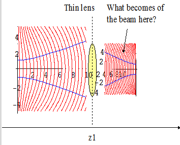
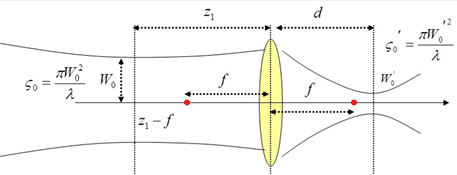
Let's set z=0 at
the waist of the input beam. Then, let’s write the input Gaussian
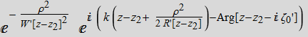
profile at ![]() just before the lens. From:
just before the lens. From:
 (2.1.2a)
to: ![]() (4.2.1)
(4.2.1)
(We drop the term 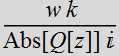 which is just an overall amplitude factor without any effect on
profile and phase for simplicity).
which is just an overall amplitude factor without any effect on
profile and phase for simplicity).
Remember that: 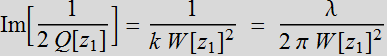 (4.2.2a)
and: 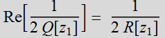 (4.2.2b)
Then, by substitute (4.2.2), (4.2.1) becomes:
 (4.2.3)
The output beam just after the lens is:
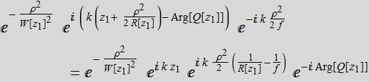 (4.2.4)
If we
define: 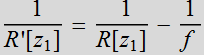 , (4.2.5)
(Note: ![]() is NOT the derivative of R[z]
at
is NOT the derivative of R[z]
at ![]() .
)
.
)
then we can
write: 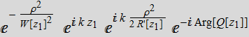 (4.2.6)
Let's look at
the expression. What does it tell us?
Obviously, it has a Gaussian amplitude profile:  ;
and a paraboloidal phase term:
;
and a paraboloidal phase term: ![]() . This is a typical Gaussian profile! (note: The phase term
. This is a typical Gaussian profile! (note: The phase term ![]() ,
like the amplitude term
,
like the amplitude term  that we drop, is ONLY a constant phase term without any
ρ-dependency hence, just a factor).
that we drop, is ONLY a constant phase term without any
ρ-dependency hence, just a factor).
The only difference between this output Gaussian and the input
Gaussian is that the phase front has a radius of
curvature ![]() instead of
instead of ![]() .
They both have the same beam spot radius at
.
They both have the same beam spot radius at ![]() :
:
![]() . Thus,
this is also a solution of the Helmholtz equation.
. Thus,
this is also a solution of the Helmholtz equation.
The output of a Gaussian beam
through a an on-axis thin lens is a Gaussian beam. BUT
this Gaussian beam is NOT the same as the input (inspite of the
fact that BOTH have the same beam spot radius at ![]() :
they have difference phase front at
:
they have difference phase front at ![]() ).
).
So, to find out the property of this output Gaussian from the
lens, we must find a Gaussian beam expression that gives us
exactly the beam spot radius: ![]() and radius of curvature
and radius of curvature ![]() at location
at location ![]() .
.
Let's write the expression again:

Now we recall that in
general, 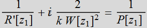 (4.2.7)
where ![]() is the Q-function (virtual point) for some Gaussian beam.
is the Q-function (virtual point) for some Gaussian beam.
How do we do that?
Basically we
must find the beam waist location ![]() and beam waist
and beam waist ![]() . We
write the general expression for a Gaussian beam:
. We
write the general expression for a Gaussian beam:
 (4.2.8)
This is expression for a beam with waist at z=0. We shift the
coordinate to ![]() :
:
 (4.2.9)
At ![]() :
:
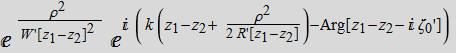 (4.2.10)
Now, this beam must match with the output Gaussian beam from the
lens at ![]() ,
right?
,
right?
So, we compare terms by terms:
1- Amplitude
profile: 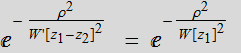 (4.2.11)
which yields:![]() ;
or:
;
or:
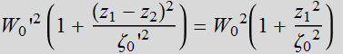
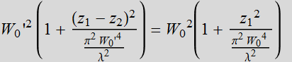
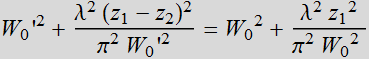
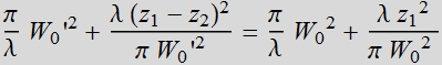
 (4.2.12)
2- Phase profile:
![]() (4.2.13)
(4.2.13)
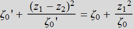
Again, separate the ρ-dependent term from the others:
 (4.2.14)
which is precisely the wavefront relation we mention earlier.
The other term is NOT important here since it is just a constant
phase shift (no ρ or z-dependence).
Recalling that 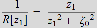 ,
we have the equation:
,
we have the equation:
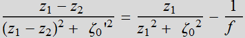 (4.2.15)
Solving the equations
Let's rewrite
the Eqs. again:
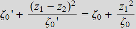 (4.2.12)
 (4.2.15)
Changing ![]()
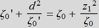 (4.2.16a)
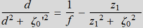 (4.2.16b)
So we have 2 eqs. with 2 unknowns.
![]()

4.3 Result discussion
4.3.1 Relations between the beams
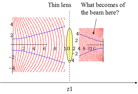

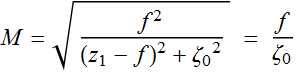
The first
result:  or (4.3.1)
 (4.3.2)
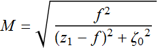
where we define:  (4.3.3)
Next:

![]() (4.3.4)
(4.3.4)
The quantity M is interesting: it is the ratio between the 2 beam
waists. Thus we define M to be the "magnification" factor (as if
we use the lens to magnify or focus the beam). We see these
relations are somewhat similar to ray-optics of lens that we are
familiar.
In fact we have other relations involving M:
Rayleigh range: 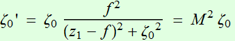 (4.3.5)
Beam divergence: 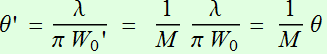 . (4.3.6)
Write a code calculate output beam waist and location as a function of input beam parameters
Transforming: Given a beam, and you wish to transform it into another beam, can you find a lens to do it (HW)
4.3.2 Meaning of the "magnification" (or reduction) term
Let's look at the term:
 (4.3.3)
If the beam is point-like: it has a small beam waist and short
Rayleigh range, then:
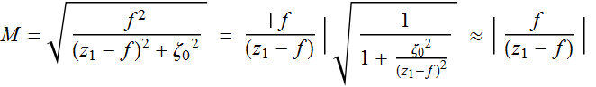 (4.3.7)
If ![]() so that
so that 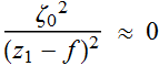 .
.
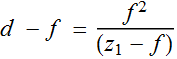
But this is the typical ray-optics lens relation:
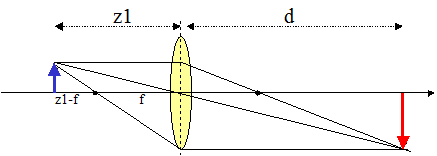
Image magnification: ![]()
In fact, we look at other relation:
![]()
or: 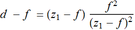
![]()
![]()
 (4.3.8)
This is the lens imaging relation in geometrical (ray) optics.
Depth of
focus: ![]() (4.3.9)
(4.3.9)
All of these relations are compatible with ray optics.
When is this concept not relevant? obviously, when the beam waist
is large: the beam is more "plane-wave" like rather than spherical
wave emanating from a spot: now we know when we can use simple
geometrical optics and when we should not when dealing with
Gaussian beam: the Rayleigh ranges << f or the waist is very
small.
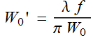
4.3.3 Gaussian beam focusing or mode matching
Now we have the other extreme: our beam is pencil
like, which means it has a large Rayleigh range: ![]() .
Also, the beam waist should also be close to the lens, in other
words,
.
Also, the beam waist should also be close to the lens, in other
words, ![]() .
What will happen?
.
What will happen?
Let's look at beam waist:
Since we assume that ![]() ,
we can write:
,
we can write:
or the famous Gaussian beam transform formula:
![]() (4.3.10)
(4.3.10)
Notice how the beam waists are inverse of each other: input a
large beam, we have a very small focused spot. Input a small spot,
we have a large focus spot.
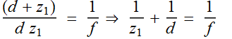
4.3.3 Focal-focal conjugate
Now suppose we want the "symmetric case". Can we
make a beam such that the input is similar to the output except
for a displacement of the waist?
What if we just put a Gaussian waist at the focal plane of a lens?
That is: ![]() or
or ![]() ?
?
From the
above: ![]()
This means that the output beam waist is at the other focal plane.
Sure, this is simple enough to understand: if we put a beam waist
at one focal plane, the lens just bend the phase such that the
output is at the other focal plane. But what happens to beam waist
size? For that, we need:
If we want the two beams also to be nearly equal in waist, we
need ![]() ,
in other words, the Rayleigh range of the beam has to be nearly
equal to the lens f. So we can't arbitrary make beams like that
for a given lens. Either we choose the lens f or we must have beam
with proper waist!
,
in other words, the Rayleigh range of the beam has to be nearly
equal to the lens f. So we can't arbitrary make beams like that
for a given lens. Either we choose the lens f or we must have beam
with proper waist!
Demo of Gaussian beam through a lens
Demo Homework lens selection for Gaussian beam transform
Consider focusing a beam:

Consider focusing. From the formula:
![]() (4.3.10)
(4.3.10)
If we want a very small focused spot, we want ![]() as large as possible. But the input beam can’t be larger that the
lens! otherwise, the power will not be collected. Hence, we can
say that
as large as possible. But the input beam can’t be larger that the
lens! otherwise, the power will not be collected. Hence, we can
say that ![]() is limited by the radius of the lens r.
Hence:
is limited by the radius of the lens r.
Hence: 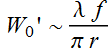
But the ratio 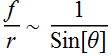 ,
which is also called nunerical aperture (NA) of the lens. We see
that it doesn’t matter large lens or small lens, the only thing
that matter is the NA:
,
which is also called nunerical aperture (NA) of the lens. We see
that it doesn’t matter large lens or small lens, the only thing
that matter is the NA:


The above 2 lenses give exactly the same spot size
when focusing:
 (4.3.11)
That’s why NA is the only rating that matter in lenses when it
comes to resolution: how fine the details we can see or how small
a spot we can focus.
4.3.4 Off-axis beam: (advanced only)
4.3.5 Linear decomposition approach
4.3.6 Numerical aperture of a lens
4.3.7 Summary
Now we know why Gaussian beam is so interesting: it remains a Gaussian (although transformed) through lenses or curve mirrors. All the above relations with lens also apply with spherical (or paraboloidal mirror).
- With appropriate conditions, we can find a set of Gaussian solutions that remain invariant in a system of optics: laser cavity or lens guide (obsolete applications).
- We'll see that Gaussian turns out to be just one solution among many cavity modes; not surprisingly, it is the simplest solution, or the lowest order solution.
- More importantly: many concepts above are NOT exclusive to Gaussian beam. Even non-Gaussian beams have similar behavior: this is because they all are governed by diffraction. What we learn is the diffraction of paraxial light beam. Gaussian is a special case.
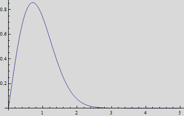
In the vertical dimension, a diode beam coming out of its facet has a flat wavefront and an amplitude profile like this:
Plot the wave profile of the beam as it leaves the diode facet along the x and z dimension. Use reasonable assumption of everything. (you must figure it out yourself).
Assignment: do all the excersizes in section 4.3 above and this:
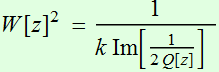
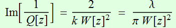
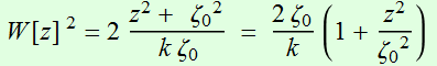
John measured a beam with a Gaussian intensity
profile  and obtained w= 2.5 μm. The wavelength was λ=1 μm. He then
measured the beam divergence which has a full width half max
(FWHM) of 35 degree. Is this posible?
and obtained w= 2.5 μm. The wavelength was λ=1 μm. He then
measured the beam divergence which has a full width half max
(FWHM) of 35 degree. Is this posible?
5. Advanced demonstration: Large NA beam