
Lightwave Polarization
ECE 5368/6358 han q le - copyrighted
Use solely for students registered for UH ECE 6358/5368 during courses - DO NOT distributed (copyrighted materials)
1. Introduction
1.0 Prolog
We know that E and H are vectors, and so far, we sometimes treat them as single-component (or scalar) for convenience. But for many optical phenomena, the vectorial nature of light is quite important. This is what we refer to as “polarization” and will study here.


Yoav Y. Schechner and Nir Karpel. Recovery of Underwater Visibility and Structure by Polarization Analysis, IEEE Journal of Oceanic Engineering, Vol.30 , No.3 , pp. 570-587 (2005).
1.1 Plane wave revisited
See Plane wave demo link.
2. Example: polarization in dipole radiation
Find a most common concept in these pictures

In the follow, skip the math if it appears too complex, focus on understanding various illustration. Understand what each graph plots and what key property it shows.
2.0 General discussion
Where do polarization come from? From the fundamental perspective of quantum theory, polarization comes from the spin state of the photon, since it is a particle with spin angular momentum J=1. But classically, we can also see where the polarization come from. A good example is the radiation from a dipole.
An excited electron (in atoms, molecules, or condensed matter) can lose its energy by emitting photons, a process known as emission. (Later on, we will learn that emission can be spontaneous or by stimulation). But a key feature of the transition is the electric moment of the transition. Most common is dipole moment, which means that the quantum mechanical transition has the classical equivalence with dipole radiation.
Semi-classical quantum description
Note: “semi-classical” because we don’t treat the photons as fully quantized field coupled with electrons but only as A.p in 
The term 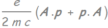 treated as
is considered as “classical” treatment of the EM field.
We will see that the momentum operator p allows transitions only between certain electronic quantum states, known as “selection rule” because of angular momentum conservation.
We know that diode lasers around us emit polarized light. Where does that come from? In fact, it comes from atomic transition as shown above.
Right around the bandgap Γ point:
- The conduction band is like an S state, l=0 and electron spin s=1/2:
 or
or 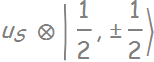 (or conduction band
 ![]() )
)
- The valence band is like a spin-orbit coupled P-state: l=1 coupled with s=1/2 to give us:
-  is known as the split-off band (pink band above)
-  consists of 4 states grouped into 2:
  : heavy hole (because its mass is usually heavier than the other 2 states), and
  : light hole states for the reverse reason.
- At k=0 (Γ point in Brillouin zone), light holes and heavy holes are degenerate: they have the same energy, but...
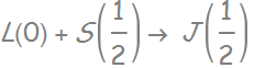
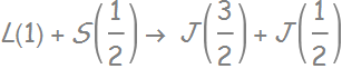
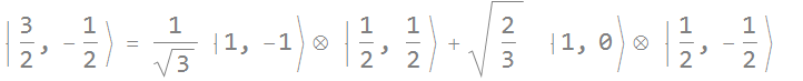
- With quantum well (or strains or any other external perturbation such as magnetic field), they separate in energy and light emitted from the condition band l=0, m=0 to heavy holes (usually the lowest energy states) or light holes (in some cases) is a dipole transition, resulting in an angular momentum change of the electron, which is imparted on the photon spin:
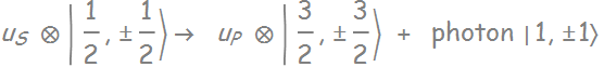 with {Δm}=1
- Linear polarization is a linear combination of {1,1> and {1,-1> also known as ![]() and
and ![]() states of the photon.
states of the photon.
Because  term, and p is in the plane of the QW, the transition E-field is parallel with the quantum well (QW) plane, we have TE polarization. When the transition dipole moment is perpendicular to the QW plane, we have TM polarization.
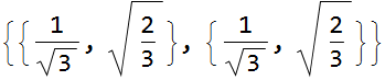
Extra note: for those who are interested, Mathematica has built in Clebsch-Gordan coefficient:
![]()
![]()
Which means simply: ![]()
These are the heave hole spin states
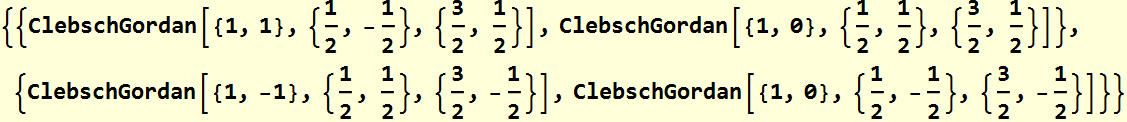
Which means simply: 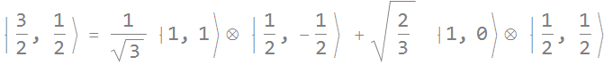
These are the light hole spin states. Transitions from conduction band electron ![]() to heavy-hole states have larger coefficients than those to light-hole states.
to heavy-hole states have larger coefficients than those to light-hole states.
Classical EM description
Classical dipole radiation is a very good simple example where polarization comes from. Also, it is a spherical wave rather than plane wave, and hence, do not associate polarization exclusively with plane wave that we happened to use as an example in previous chapters.
We will see that in the farfield, plane wave approximation can be applied locally on a point on the wavefront. Here, we will see how plane wave polarization we learn previously is connected to the dipole radiation we are studying here.
Here, the polarization comes from the source dipole. It is intuitively obvious: if the electrons oscillate along an axis, we would expect the E field should be oriented along the same axis. In addition, we know that the field should be perpendicular to propagation vector k. Thus, we infer that the polarization should be along the axis that is the intercept of the 2 planes: the plane containing the dipole and the plane perpendicular to k.
Indeed, this is the case.
2.1 Classical dipole radiation fields and power
We don’t have to get into details here (see chapter on scattering and dipole scattering), but it is sufficient to summarize key properties and see illustration to gain insight on polarization.
In quantum mechanics (not this course), we will learn that the semi-classical field for the transition is the A . p
The radiating magnetic field from a dipole is: 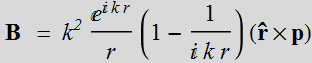
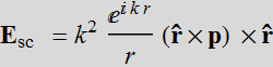
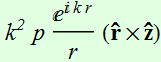
The electric field is: 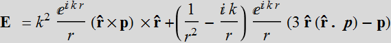
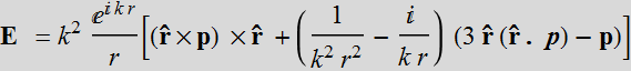
Far field scattering: k r is very large k r >> 1
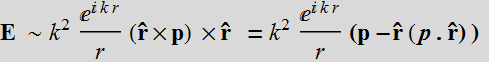
Note that: ![]()
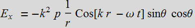
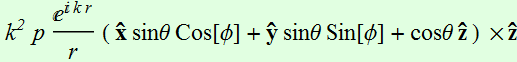
Let p be in the z direction, then: 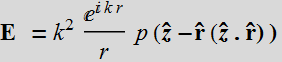
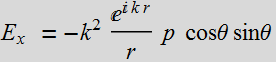
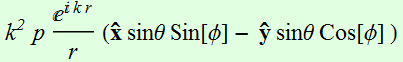
Take the real part: 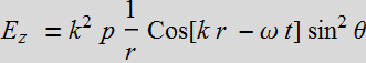
Let's look at the Poynting vector of the radiation field: 
since ![]() as E is orthogonal to
as E is orthogonal to ![]() (
( )
)

Thus, the Poynting vector is just a spherical outward field:
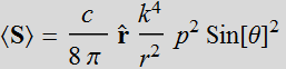
that has a simple angular dependence: ![]()
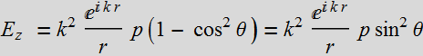
2.2 Dipole radiation intensity pattern
From the above, in the FF, the dipole radiation is essentially a spherical wave.
But its power is NOT directionally uniform.
The power density radiation FF pattern is simply:
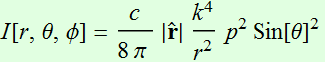
![]()
This is the radial plot of intensity: it is strongest at the belly (equator) and zero at the north and south poles.  Note how similar it is to Cos[θ] law of incident power.
This is another plot of the time-averaged Poynting vector in a vertical plane (meridional plane).
In the FF, the dipole is just like a point source and the phasefront is spherical as shown. However, notice the plot shows that the intensity (vector length), is large at the equator and decreases toward to the poles.
2.3 Dipole E field
2.3.1 Vectorial plot of E field
As discussed above:

The E field is always along the North-South line.
Demo dipole E field meridional plane
2.3.2 Amplitude of E field
Demo E field density plot
2.4 Dipole H field
In the far field: 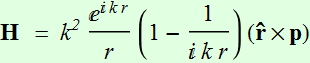 ~
~ 
~ 
~ 
H is ONLY in plane parallel to x-y, in other words, it is always parallel to the equatorial plane.
Demo H field equatorial plane
Additional simulation
2.5 Both E and H
![]()
Regardless of the exact nature of a phasefront, if λ << than the phasefront curvature at a local point, the polarization at that point can be thought in terms of that of a plane wave that is tangential to the phase front at that point.
3. General theoretical polarization description
3.1 General expression
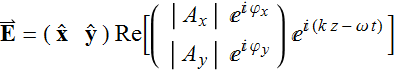
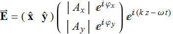
In general, for plane wave or where we can approximate as a plane wave (in the tangential plane to a phasefront), we can choose locally z-direction to be along ![]() , then, the electric field can be written:
, then, the electric field can be written:
![]() (3.1.1a)
(3.1.1a)
where ![]() is a vector that can be projected in a Cartesian coordinate system of the tangential plane, which is x-y plane:
is a vector that can be projected in a Cartesian coordinate system of the tangential plane, which is x-y plane:
![]() =
= ![]()
![]() +
+ ![]()
![]() (3.1.1b)
(3.1.1b)
Obviously, we may ask, why not choosing either ![]() or
or ![]() to be along
to be along ![]() so that
so that ![]() becomes single component?
becomes single component?
The problem is, why do we assume that ![]() and
and ![]() are real? Because only then, we can choose an angle φ such that:
are real? Because only then, we can choose an angle φ such that:
 (3.1.2)
and by rotating the x-y axis by φ, we can have a new coordinate such that ![]() is along the new axis x.
is along the new axis x.
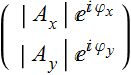
But if we have to express ![]() in the most general way, we should write:
in the most general way, we should write:
![]() = |
= |![]() |
| ![]() ;
; ![]() = |
= |![]() |
| ![]() (3.1.3)
(3.1.3)
then ![]() = (
= ( ![]() |
|![]() |
| ![]() +
+ ![]() |
|![]() |
| ![]() )
) ![]() (3.1.4a)
(3.1.4a)
or ![]() = (
= ( ![]() |
|![]() | +
| + ![]() |
|![]() |
| ![]() )
) ![]() (3.1.4b)
(3.1.4b)
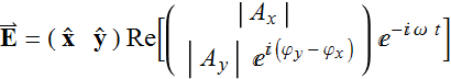
Notice that only the phase difference ![]() matters, because
matters, because ![]() is just an arbitrary phase term that can be added to the common term
is just an arbitrary phase term that can be added to the common term ![]() which can be made equivalent with a translation of z origin or a time origin shift.
which can be made equivalent with a translation of z origin or a time origin shift.
If ![]() , we can’t rotate the x-y axes in such a way that
, we can’t rotate the x-y axes in such a way that ![]() will be along either the new
will be along either the new ![]() or
or ![]() .
.
What happens to the polarization if ![]() then?
then?
In the following demonstration, we define ![]() , to designate as the retard phase, such that negative φ or Δφ means “late”, “retard” and positive phase means “early” or “advance” of y component relative to x. It is like an airplane is scheduled to arrive at 8:00 AM, but is late and arrives 8:20 AM. Then the time discrepancy: 8:00 AM- 8:20 AM = -20 minutes is the loss time and negative. The opposite is extra time gain and positive.
, to designate as the retard phase, such that negative φ or Δφ means “late”, “retard” and positive phase means “early” or “advance” of y component relative to x. It is like an airplane is scheduled to arrive at 8:00 AM, but is late and arrives 8:20 AM. Then the time discrepancy: 8:00 AM- 8:20 AM = -20 minutes is the loss time and negative. The opposite is extra time gain and positive.
Demo basic polarization
3.2 Circular polarization
If φ=0, we have linear polarization as seen above. Linear polarization may appear most “natural” to us.
Yet, from the more fundamental perspective of quantum theory, photon is a spin-1 particle with angular momentum J=1. But having zero rest mass, it can have only 2 spin states ![]() =+- 1. For a monochromatic plane wave moving in z-direction, the eigen-spin-state for J projected along the k-vector axis corresponds to either right-handed circular polarized wave (
=+- 1. For a monochromatic plane wave moving in z-direction, the eigen-spin-state for J projected along the k-vector axis corresponds to either right-handed circular polarized wave (![]() =+1) or left-handed circularly polarized wave (
=+1) or left-handed circularly polarized wave (![]() =-1) .
=-1) .
What is exactly “circularly” polarized wave? We can see it in the follow by illustrating the general expression in Eq. (3.1.4)
Imagine we are at z=0 (choose z=0 at the point of observation). Then, we look straight into the lightwave as the wave is coming straight to us, into our eyes.
Demo circular polarization
What we see here is that ![]() traces out a circle, rotating counterclockwise This is the case for |
traces out a circle, rotating counterclockwise This is the case for |![]() |= |
|= |![]() | and
| and ![]() .
.
Now, choosing ![]() , and keep |
, and keep |![]() |= |
|= |![]() | We see that it also traces a circle, but rotating clockwise!
| We see that it also traces a circle, but rotating clockwise!
Indeed, these are the two spin states of a photon. The convention we use here will be that the counter clockwise (looking at source) is called right-handed circular polarization, or positive, or ![]() polarization. The clockwise is called left-handed circular polarization, or negative, or
polarization. The clockwise is called left-handed circular polarization, or negative, or ![]() polarization.
polarization.
See more illustration in HW: circular polarization ![]()
3.3 General elliptic polarization
But in general, the phase difference can have any arbitrary value, not just ± π/2, and |![]() |≠ |
|≠ |![]() |. We can see what happens:
|. We can see what happens:
Demo general elliptic polarization
If Δφ=0 or ± π, we have linear polarization, as expected.
More generally, we can have any shape of ellipse. this is called elliptic polarization. 
We can see the general ellipse form in the follow.
First, note that another way to express ![]() is using vector dot product notation:
is using vector dot product notation:
 (3.3.1)
Later, we will see this is also useful dealing with polarization changes through different optical elements.
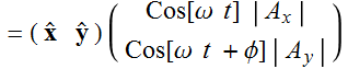
At a fixed z position, such that ![]() , the ellipse is swept by the parametric plot of the E field for a as time varies:
, the ellipse is swept by the parametric plot of the E field for a as time varies:
Or: 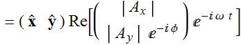 (3.3.2)
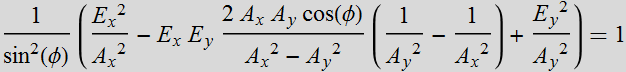
It is straight-forward algebra (substitute Cos[ω t]) to reduce the relations:
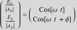 (3.3.3)
to the form: 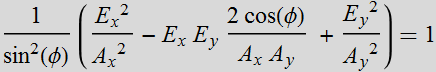 (3.3.4)
Or: 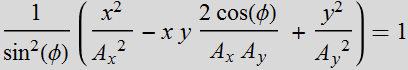 (3.3.4a)
which we can recognize as an ellipse. Another form is:
 (3.3.5a)
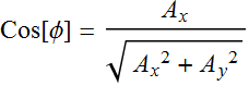
which gives us angles υ and υ+π/2 that the two ellipse principal axes make with the x-y axis:
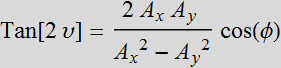 (3.3.5b)
The two ellipse axes are plotted as the blue lines in the figure, and the two principal-axis components are shown as green and orange vectors.
But then, it is clear that elleptic polarization is the most general polarization since linear and circular are only 2 extremes of an ellipse: linear corresponds to an ellipse with zero minor axis and circular is an ellipse with equal axes.
Let ![]() , Then it is clearly linear polarization:
, Then it is clearly linear polarization:
![]() = (
= ( ![]() |
|![]() | +
| + ![]() |
|![]() | )
| ) ![]() (3.3.6)
(3.3.6)
The E field makes an angle ArcTan[|![]() |/|
|/|![]() | ] with the x axis. Linear polarization is also called P-polarization or π-polarization.
| ] with the x axis. Linear polarization is also called P-polarization or π-polarization.
Let |![]() | = |
| = |![]() | = |A| ; and
| = |A| ; and 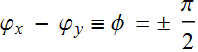 , then:
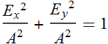 (3.3.7)
which is indeed a circle, which is circular polarization.
Demo general elliptic polarization (repeat and review)
4. Polarization in empirical description and measurements
4.1 Discussion
Based on what we see in Section 3, what should we expect light around us and in various systems? Should every light be elliptically polarized, which can also be linear or circular in special cases? Also, how do we determine and measure the polarization of light?
As it turns out, we might be surprised that notwithstanding what we said in 3.3, we will find there is such a thing as “unpolarized light”: light without any polarization at all.
How can that be? Light wave must have vector E field, and it must have polarization, so how can light NOT have polarization, to be “unpolarized”?
The answer is that in practice, we deal with light composed of many many light waves. And when we say “polarization” of a light, we are not referring to the fundamental polarization of each component of that light, but the statistical ensemble average of all the components of that light.
Every component of a light, every photon must have a state of polarization, which is a linear combination of 2 fundamental states:
![]()
Here, we use the quantum notation of {p> in order to emphasize that any photon, fundamentally must have a polarization state.
But unless we look at a light source from a quantum transition with a definite a selection rule and definite polarization state, the light around us is comprised of an infinitely large numbers of photons from many different sources that have all different frequencies, phases, and polarizations and hence, as we take the time average, there is no dominant polarization and we say that the light is unpolarized - in the statistical sense.
An analogy is that every person is either male or female. If we take a group of people, say beer drinkers, we might say there are more males than females and the population may have a gender bias such as predominantly male. But if we take a group of people in a given town with sufficiently large population, we find out that there are statistically equal number of males and females, and hence, the population is neither male nor female. This is the same as saying some light is unpolarized, because on the average, all the polarizations of all the photons cancel each other out, resulting in no net electric field in any particular polarization in time average.
Below is an illustration.
Demo random polarization ensemble
Consider the ensemble-averaged polarization vector (black) as we increase the number of fundamental linearly polarized light wave, but the polarization vector is random.
It is crucial for us to distinguish “polarization” as a fundamental property of photon vs “polarization” as an empirical concept to describe the ensemble and time-averaged of all photons of a source of light. Thus, as we say some light is unpolarized or partially polarized, we do not mean that each photon of that light does not have polarization, which is false. We only mean that the average of all photon polarizations result in either no particular measureable polarization, or some polarization. (see example below).
Here is an example of “partially linear polarized light”
Demo partially polarized ensemble
Notice that there is a preponderance of light with polarization along the vertical plane, hence, the ensemble-average polarization is not zero, but has a finite value in the vertical plane. Partially polarized light is simply light that has a distribution with a dominant state of polarization than others.
4.2 Practical measuring and effecting polarization
How do we determine light polarization?
The only way to know the polarization of a photon, is to destroy it, or its coherent partners if the photons are in a coherent state. That’s the measurement process. But if the source of photons can reliably produce similar photons, such as a stable laser, then we can say what we measure is likely also the polarization of all photons from that source.
Again, quantum theory consideration revisited
Can we determine the spin state, i. e. polarization ![]() or
or ![]() a photon? Yes. Well known in atomic spectroscopy is the principle of conservation of angular momentum. A photon absorbed or emitted as an electron makes a transition between 2 states much make up for the change of angular momentum states of the electron.
a photon? Yes. Well known in atomic spectroscopy is the principle of conservation of angular momentum. A photon absorbed or emitted as an electron makes a transition between 2 states much make up for the change of angular momentum states of the electron.
Thus, a transition involving a difference of ![]() will require the absorption or emission of a
will require the absorption or emission of a ![]() or
or ![]() photon. Note that the arbitrary convention of
photon. Note that the arbitrary convention of ![]() or
or ![]() doesnot imply any abiguity here. Usually, the transition of
doesnot imply any abiguity here. Usually, the transition of ![]() requires an external field, often magnetic field to plit these levels. The axis of the field and the spin state energy levels define the axial geometry (a reference axis that the angular momentum is projected on) and the transition and the photon
requires an external field, often magnetic field to plit these levels. The axis of the field and the spin state energy levels define the axial geometry (a reference axis that the angular momentum is projected on) and the transition and the photon ![]() or
or ![]() corresponds to actual photon spin state that is defined by the same axial geometry.
corresponds to actual photon spin state that is defined by the same axial geometry.

Technology involving light polarization
But doing spectroscopy such as magnetic resonance is not practical. The most common and familar approach is to use linear polarizer, often made with highly elongated molecules. See various illustration below. (explanation in lecture).
The molecules can be controlled externally and have interesting behavior between crystalline phase and liquid phase: liquid crystal used in LCD (liquid crystal display).


However, not all polarization-effective devices involve special molecules or materials. Many simple optical phenomena have polarization effects as we will learn, and these effects can be applied to make polarization devices.
Most common polarization optical devices perform these functions (we will learn how they work later):
- Linear polarizer: discussed above: give linearly polarized output.
- phase plate retarder: this is a birefringence material that has anisotropic dielectric constant: different polarizations have different indices of refraction. Thus light sent through such a device has a linear component, such as ![]() delay compared with
delay compared with ![]() , in other words, it acquires a phase difference compared with
, in other words, it acquires a phase difference compared with ![]() after getting through the device, 2 most common retarders are:
after getting through the device, 2 most common retarders are:
a- Quarter-wave plate, which has a phase shift of π/2 (which is λ/4, hence, called quarter-wave). Convert LP into CP (HW) (and the reverse). (Give elliptically P light if not oriented at 45)
b- Half-wave plate, or λ/2, has a phase shift of π. Rotate the LP by 90. (Give elliptically P light if not oriented at 45)
- Fresnel Rhomb: can introduced a phase shift similarly to phase plate retarder above.
- There are other more complex devices for applications such as optical fiber communications.
λ/4: 
λ/2 

Most of the time, we measure only intensity, (unless doing heterodyne detection) hence, we have to infer the polarization property of light by a number of measurements, using devices as mentioned.
4.3 Stokes parameters (or Stokes vector)
Sir George Gabriel Stokes, 1st Baronet
13 August 1819 – 1 February 1903
To appreciate Stokes parameters, let’s imagine the following: we have a bunch of polarizing filters (such as those above) and can measure only the intensity of light. We want to know the polarization property of some light, how would we measure and determine?
Demo Stokes vector concept - intro
First, suppose we have the case below. Suppose we have LP light. Let’s use linear polarizers. If we use one, what happens if it is accidentally placed perpendicular to the light P? Well, we can use 2 to put them perpendicular to each other as shown below.
First, we can measure the power (or intensity) of LP at position 0 degree: ![]() , and at 90 degree:
, and at 90 degree: ![]()
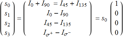
The total intensity is: ![]() : (4.3.1)
: (4.3.1)
This is the first Stokes parameter.
If there is a difference between the power for![]() LP and
LP and ![]() LP, we can tell that there is some polarization.
LP, we can tell that there is some polarization.
If there is LP, we should see a big difference between ![]() and
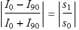
and ![]() . Hence, the second Stokes parameter is defined to measure the difference between them:
. Hence, the second Stokes parameter is defined to measure the difference between them:
![]() . (4.3.2)
. (4.3.2)
But we should normalize this quantity relative to the total power, which is:
 (4.3.3)
If this quantity =1, the light is 100% linearly polarized along one of the chosen axis. But if it is zero, what can we tell? Does it mean the light is totally unpolarized?
we see that: ![]() in this case.
in this case.
Clearly, we would be wrong to jump to such a conclusion. So, how do we deal with this?
More LP please!
By adding LP measurement along 45 and 135 degree, we cover all bases for LP. If one pair can’t tell the difference, the other pair surely would measure the maximum. Thus, we define the 3rd Stokes parameter:
![]() . (4.3.4)
. (4.3.4)
and let’s write all parameters so far:
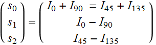 (4.3.5)
We can determine exactly the LP angle relative to our coordinates with these measurements. Note that we don’t care about the orientation of the LP’s: we can place them in anyway and never have to worry not able to detect linear polarization.
In other words, we can determine for sure how much polarization the light has. Can we really?
Demo Stokes vector concept - circular
We see a problem here:
If we have circular polarization, we will have: ![]()
Hence: 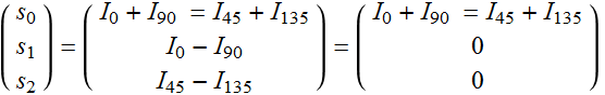 (4.3.6)
In fact, we can have 100% CP polarization but has no evidence of it!
The reason... is that we only measure LP so far!
Hence, we will need one more parameter:
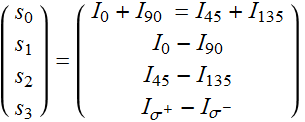 (4.3.7)
This is the Stokes parameters, which can also be treated as a vector.
HW: Write an expression for the Stokes vector of general elliptically polarized light. Find the case for LP (states), CP (2 states) as the limit of the general elliptical polarization.
What happens if we have light that is 100% of the same polarization?
We will see that: 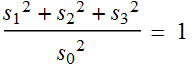 (4.3.8)
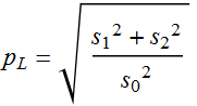
That is the reason we define the quantity:
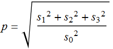 (4.3.9)
to be the “degree of polarization” of a light, abbreviated as DOP.
Note: Some convention defines
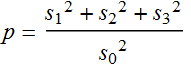 (4.3.10)
but this expression is quadratic of intensity, while (4.3.9) is linear with respect to intensity.
If the light is made up of components that have completely random polarization relative to each other, that is given any polarization, the % of light with opposite polarization is equal to each other, then the Stokes vector is:
 ; and p=0 (4.3.11)
This is what we called totally “unpolarized light”.
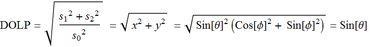
Note: a sub-concept of DOP is DOLP: degree of linear polarization
 (4.3.12)
When DOP or DOLP >0 but <1, we say the light is “partially polarized”. We can say the fraction (“percentage”) of polarized light is p, or the % of LP is ![]() .
.
4.4 Decomposition and Poincaré sphere
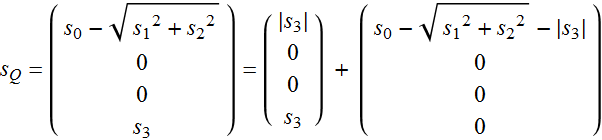
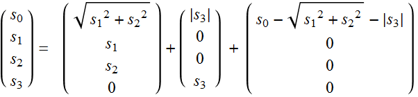
When the light is partially polarized, it must have polarized and totally unpolarized components. Hence, one way to express this idea of separating them out is:
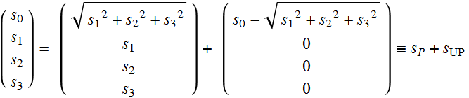 (4.4.1)
For the polarized component, a way to represent what it looks like is to use Poincaré sphere representation. The idea is simply to transform the normalized vector 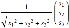 into a point on a sphere:
You can also see another representation below. But note that this representation DOES NOT relate the actual amplitude and phase of light component ![]() ,
, ![]() to a point on the sphere like ours does. It uses DoP and ellipse angle that must be measured as input. Ours is more fundamental.
to a point on the sphere like ours does. It uses DoP and ellipse angle that must be measured as input. Ours is more fundamental.
http://demonstrations.wolfram.com/LightPolarizationAndStokesParameters/
Since ![]() , when θ=0 or π (the point at north or south poles) it means that the polarization is 100%
, when θ=0 or π (the point at north or south poles) it means that the polarization is 100% ![]() or
or ![]() . At θ=π/2 (the equator),
. At θ=π/2 (the equator), ![]() , which means there is no CP whatsover in the light, which means the light is 100% linear. Note the relationship that:
, which means there is no CP whatsover in the light, which means the light is 100% linear. Note the relationship that:
 (4.4.2)
Hence, it is opposite to ![]() . The equator corresponds to max DOLP=1.
. The equator corresponds to max DOLP=1.
For the azimuthal angle φ: 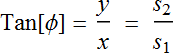 , which can be shown to be:
 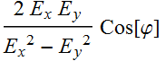 where φ is the phase difference between
 ![]() and
and ![]() . This is twice the angle of the ellipse major axis relative to the x-axis.
. This is twice the angle of the ellipse major axis relative to the x-axis.
The usefulness of Poincaré sphere is that by looking a point on the Sphere, we can immediately visualize the state of polarization: near equator: LP, near the poles: CP. In between: EP. The azimuthal angle itself is not very fundamental, since it is only relative to one of the axis we initially set as the axis for ![]()
![]() axis).
axis).
A further note. Eq (4.4.1) above is not the only way of separating polarized and unpolarized light. For example, supposed we are interested only in LP light. We can define a Stokes vector:
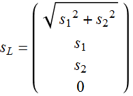 (4.4.3)
The remaining component is:
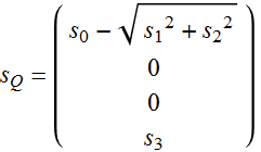 (4.4.4)
Of course, we can again separate ![]() :
:
 (4.4.5)
Hence:
 (4.4.6)
Thus, in principle, we can measure different polarized components of a source of light.
Some illustration: polarization imaging research
Link to Yi and Yang research. Mueller scattering matrix.
5. Jones vector & matrix
5.1 Polarization state and Jones vector.
Polarization states belong to a two-dimensional space and any 2 linearly independent vectors can form a basis set. The two most natural bases are linear polarization and circularly polarization.
We implicit use linear polarization basis in Section 3 above by expressing the E field in terms of orthonormal basis ![]()
 (3.3.1) (5.1.1)
The light instantaneous intensity is proportional to:
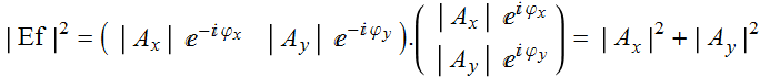 (5.1.2)
We describe the polarization state of an electric field with
 , or
, or 
 (5.1.3)
which, we refer to as a Jones vector.
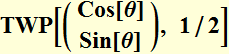
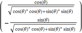
Examples: vector  is linear polarization along x axis (the ± sign is not important).
 is linear polarization along y axis.
  is linear polarization making an angle θ with x axis.
How would we describe a circular polarization?
We see clearly that the requirement for ![]() is:
is:
|![]() | = |
| = |![]() | = |A| ; and
| = |A| ; and  . Thus:
A ![]() -state is
-state is 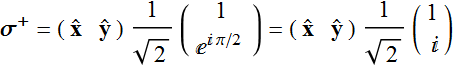 ; (5.1.4a)
and a ![]() -state is
-state is 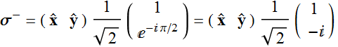 ; (5.1.4b)
These two states are clearly orthonormal by taking their dot product:
 (5.1.5)
We can see 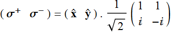 ; (5.1.6)
Or: 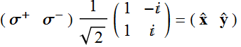 (5.1.7)
Hence, we can convert a Jones vector in the linear polarization basis to that in the circular polarization basis and vice versa with the transformation:
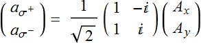 (5.1.8a)
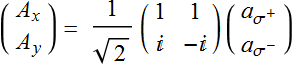 (5.1.8b)
Of course we can make any arbitrary basis with any non-singular transformation matrix.
What is the use of this description? We will see that it can help tracking the polarization of light as it goes through a device or system. A device effect on polarization can be described with a matrix, and the output is simply a transformation of the input Jones vector by the device matrix.
5.2 Jones matrix
5.2.1 Definition
As light goes through an optical device, from something as simple as the reflection from an interface of a dielectric, the transmission through a thin optical film, or through an optical fiber, a waveguide modulator... (more about this topic later on), its polarization usually changes. The change is usually a linear process and thus, can be expressed as a matrix transformation.
A most general expression is:
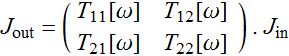 (5.2.1)
Because most optical devices have frequency-dependency, we include the ω term. But for simplicity, we can drop it here. The matrix: 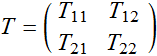 (5.2.2)
is called the Jones matrix. It represents the effect of the device on the state of polarization vector.
A system may have several devices, hence, the effect of the polarization can be obtain by simply multiplying the Jones matrix for each device sequentially:
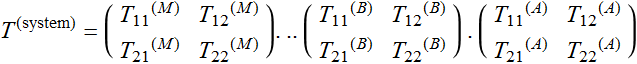 (5.2.3)
5.2.2 Common examples
For a linear polarizer plate, it absorbs almost all light in one axis and transmits light on the other axis. The Jones matrix is:
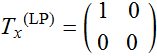 ; or
; or 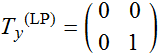 (5.2.4)
which shows the absorption on the y-component or x-component polarization.
For wave retarders, the Jones matrix here is:
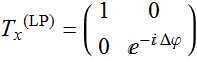 (5.2.5)
which shows a differential phase shift Δφ between the two polarizations.
As discussed above, if Δφ = -π/2, it’s called a quarter-wave retarder,
if φ = -π it’s called a half-wave retarder
Example: Define:

as the Jones matrix of a phase plate of 2 π φ retardation of the y -axis.
Thus, if we input a LP at 45 degree of a λ/4 wave plate:

which is a circular polarization ![]() . We can illustrate as follow:
. We can illustrate as follow:
Demo polarizer plate with retarded axis
input: linear pol (green); output: ![]() or
or ![]() (red), depending which input angle (45 or 135). This is for λ/4
(red), depending which input angle (45 or 135). This is for λ/4
We see that a P-wave 45 degree with the axis through a 1/4-wave plate is transformed into either ![]() or
or ![]() depending on
depending on
 or
or 
If input angle θ is different from a multiple of 45 degree (π/4), it will give an elliptic polarization:
For the below, we see that a P-wave 45 degree with the axis through a 1/2-wave plate is flipped across an axis, resulting in 90 degree rotation:

![]()

More generally,


5.2.3 More general consideration
It may appear that the Jones matrices for many simple optical devices are diagonal:
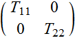
but that is not true generally. Actually, mode coupling, which involves off-diagonal terms ![]()
![]() are quite common, such as waveguides, or devices that light bounces more than once, or devices without a certain principal plane that preserve the separation of polarization such as transverse electric (TE) and transverse magnetic (TM). In addition, a diagonal matrix in one basis, such as LP, is not necessarily diagonal in another basis such as CP. Lastly, a real system with combination of multiple devices would likely have polarization cross coupling.
are quite common, such as waveguides, or devices that light bounces more than once, or devices without a certain principal plane that preserve the separation of polarization such as transverse electric (TE) and transverse magnetic (TM). In addition, a diagonal matrix in one basis, such as LP, is not necessarily diagonal in another basis such as CP. Lastly, a real system with combination of multiple devices would likely have polarization cross coupling.
Consider for example, the reflection from a perfect metal.
Again, the Jones matrix is diagonal. But let’s see what happens if we use the basis of CP.
From Eq.
 (5.1.8a)
 (5.1.8b)
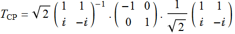 (5.2.6)
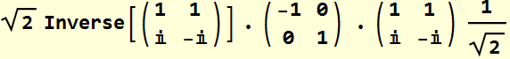
Thus:  (5.2.7)
which have off-diagonal elements. This means that an input ![]() will become output
will become output ![]() and vice versa.
and vice versa.